# Run this cell before beginning the exercises.
# You may need to select a kernel for the notebook -> TheGuide

# package imports (SHIFT + ENTER to run)
import numpy as np
import matplotlib.pyplot as plt
from matplotlib.patches import Circle, Ellipse
import ipywidgets as widgets
from ipywidgets import interact
from IPython.display import YouTubeVideo
from IPython.display import HTML, display
from typing import List, Tuple, Optional, Union
Introduction#
Hello Microlenser. I am your Guide.
I'll keep this introduction brief, in case you are short on time.
This notebook is going to take a leisurely stroll through the "basic" concepts of microlensing. This topic is complex and has a lot of nuance, so I propose we first familiarise ourselves with the scientific motivations, background information, and key discoveries (the stuff that doesn't make us want to bang our heads against the wall) and get to know each other a little. But if that doesn't sound like somthing you want to do, I'm not offended; I'm a notebook.
Below is a list of the concepts we will cover in this introduction. However, it has been broken up in to 4 parts (with this being part 1) to make the whole thing a more managable task. Feel free to skip to whatever point makes you feel good. Or skip the whole introduction series by going straight to the Next steps section and picking out your next notebook from there.
Contents
What is microlensing? (part 1)
There are walls of text coming up, and if you are not ethused by that, I get it. Consider watching this introductory lecture by Rachael Street (author of Microlensing Source), from the 2017 Sagan Summer Workshop, instead.*1
*1 The slides are not stepped through at the correct times in the video, but they are available here.
If you take that route, it may still be worth browsing the activities in these notebooks to help build your intuition and code base. For example, there are some interactive plots in this section, python querries of the NASA Exoplanet Archive in this section, reading and visualising data from csv files in this section, python queries of Simbad and json file usage in this section.
All of the exercises are meant to help build you intuition for microlensing, but they also provide a variety of examples of different analysis and visualisations you can perform with python. As always with these notebooks, it is intended that you skip content as you see fit. If doing the python exercise is not something that floats your boat, you can always use the model code in the Exercises subfolder to see the intended results. Similarly, they are there to help you if/when you get stuck.
Okay, let's meander a bit. This notebook will make use of a variety of media to keep it accessible and interesting for all users. And, if you need some motivation, or dopamine throughout, take a look at the checklist tool where you can tick off sections for this, and other, notebooks as you complete them.
Here is a cozy little youtube video to get us in to the mood for learning about microlensing (and also to check that I'm running correctly).
YouTubeVideo('VeAVmp9MLH4', width=560, height=315)
The above video may not work for you if you are using an IDE. Try clicking this link to open it in a browser. We will provide links, like that, for all embedded videos in these notebooks.
If you are still having issues, consider opening this notebook in a browser by running
(TheGuide) Notebooks$ jupyter notebook
or (recommended)
(TheGuide) Notebooks$ jupyter lab
in a terminal, from the Notebooks directory, with the provded environment activated.
The part in brackets (
(TheGuide)) tells us the environment we have activated and the part before the dollar sign (Notebooks$) tells us what folder, or directory, we are in.
Gravitational lensing is a strange and fascinating phenomenon in astrophysics and a uniquely powerful tool for unveiling the secrets of the universe. At its core, this phenomenon is rooted in Einstein's theory of general relativity. It occurs when the gravity of massive objects, such as galaxies, stars, planets, or dark matter, curves spacetime, distorting the path travelled by light as it passes by, as if the light were passing through a lens. This can make the objects producing this light (the sources) appear to be in locations they are not and as shapes they are not. If the visible source is approximately behind a simple lensing mass, as seen by an observer, the source will be observed as a magnified image, or images, of itself. These images will form about the Einstein ring and will often appear stretched and curved. The radius of this ring, \(\tilde{r}_E\), is dependent on the mass of the lens; a greater mass results in a larger Einstein ring.
Microlensing Source has an excellent glossary of microlensing variables, for when you inevitably lose track of them all. We have included a pdf version in the 'GuideEntries' directory, should you require it.
The angular Einstein radius is defined by,
where \(M_{\rm L}\) is the total mass of the lens system, \(D_{\rm LS}\) is the distance from the lens plane to the source plane, \(D_{\rm L}\) is the distance from the observer to the lens plane, \(D_{\rm S}\) is the distance from the observer to the source plane, and \(\kappa=4G/(c^2\rm{au})\sim8.14 \, \rm{mas}/M_\odot\).
Refer to Microlensing Source for a detailed explanation of how this Einstein ring equation in derived.
Below we define a python function for this angular Einstein ring size. The units for this can be a little bit tricky to get right, so take care when defining your own functions.
def theta_E(M: float, Dl: float, Ds: float) -> float:  # this is a function definition with a type hint
    """
    Calculate the Einstein radius of a lensing system.

    Parameters
    ----------
    M : float
        Mass of the lens in solar masses
    Dl : float
        Distance to the lens in kpc
    Ds : float
        Distance to the source in kpc

    Returns
    ----------
    float
        Einstein radius in arcseconds

    Notes
    ----------
    The Einstein radius is calculated as:
    ``` math::
    theta_E = sqrt(4 * G * M / c^2 * (1.0 / Dl - 1.0 / Ds)
    ```
    where
    - G is the gravitational constant
    - M is the mass of the lens
    - c is the speed of light
    - Ds is the distance to the source
    - Dl is the distance to the lens.
    """

    # Constants
    kappa = 8.144  # mas/M_Sun
    #kappa_mu = kappa*1000  # muas/M_Sun
    #as2muas = 1.0*1000000.0  # 1 as in muas
    as2mas = 1.0*1000.0  # 1 as in mas

    # Calculate Einstein radius
    pirel_as = (1./(Dl*1000)-1.0/(Ds*1000))
    pirel_mas = pirel_as*as2mas
    #pirel_muas = pirel_as*as2muas
    #print(pirel_as, pirel_muas)
    return np.sqrt(kappa * M * pirel_mas)
This ring is a mathematical construct, but the figures below show some pretty examples of the Einstein ring being observed as it is traced out by source images during gravitational lensing events.
HST images of gravitational lensing |
|---|
|
"The Molten Ring” - GAL-CLUS-022058s. This image depicts a fairly complete Einstein ring around a spherical lensing galaxy, with minor distortions for foreground galaxies. Credit: ESA/Hubble & NASA, S. Jha Acknowledgement: L. Shatz. |
|
“A smiling lens.” This image shows another example of strong gravitational lensing where the image formed about the Einstein ring appears like a mouth under the two "eyes" made from nearby elliptical galaxies. Credit: NASA & ESA Acknowledgement: Judy Schmidt. |


1. What is microlensing?#
Microlensing is a specific example of gravitational lensing, where the apparent separation of the lensed images is small enough (i.e., microarcseconds) that they cannot be resolved into individual images with current technology.
In photometric observations, this means that the entire "strong" lensing effect is contained within what appears to be a single star or point-spread function (PSF). The lensing can instead be observed because of the changing magnification and number of source-star images creating variations in brightness. The brightness increase is transient in nature as the lens and source are moving relative to each other. This effect is called photometric microlensing.
In bouts of hubris, unbecoming of a notebook, I will often refer to photometric microlensing as simply microlensing. Astrometric microlensing is a topic left out in the cold for the duration of this notebook (my apologies to all the astrometric microlensing Stans), but should you wish to show it some love, you can do so here.
If we could see the magnified images in a microlensing event forming, they would shimmy around paths that trace out the Einstein ring. The event would look something like this:
Theoretical peak magnification \(A_{\rm peak}\), for a simple microlensing event, occurs when the lens and source are most closely aligned, with an angular separation of \(u_0\), at time \(t_0\). The intensity of an event's \(A_{\rm peak}\) depends on how closely the source aligns with the lens (i.e., how small \(u_0\) is) and the angular size (\(\rho\)) of the source, proportional to the angular size of the Einstein ring, \(\theta_{\rm E}\). The time taken to change lens-source relative positions by \(\theta_{\rm E}\) is \(t_{\rm E}\). Therefore, \(t_{\rm E}^{-1}\) can be used as a proxy for lens-source relative proper motion;*2
*2 Note that, in this equation, \(\mu_{rel}\) is in the reference frame of the observer. So, if the observer is on Earth, that is \(\mu_{rel,geo}\).
The dependence of magnification on angular-separation is demonstrated in this figure.
|
|---|
Left: Example trajectory diagram in the lens plane, showing set of source trajectories (purple) with varying \(u_0\). The lens object position is plotted as a red, filled circle. The scale of the caustic diagram is in units of \(\theta_{\rm E}\), and the Einstein ring, about which source images form, is indicated by the dashed grey circle. The angular source size (\(\rho=0.05\)) and relative trajectory direction are indicated by the circle and arrow on the trajectory lines, respectively. Right: Corresponding magnification curves, given the trajectories shown on the diagram (left), where \(\tau\) is the time, relative to \(t_0\), scaled by \(t_{\rm E}\). |
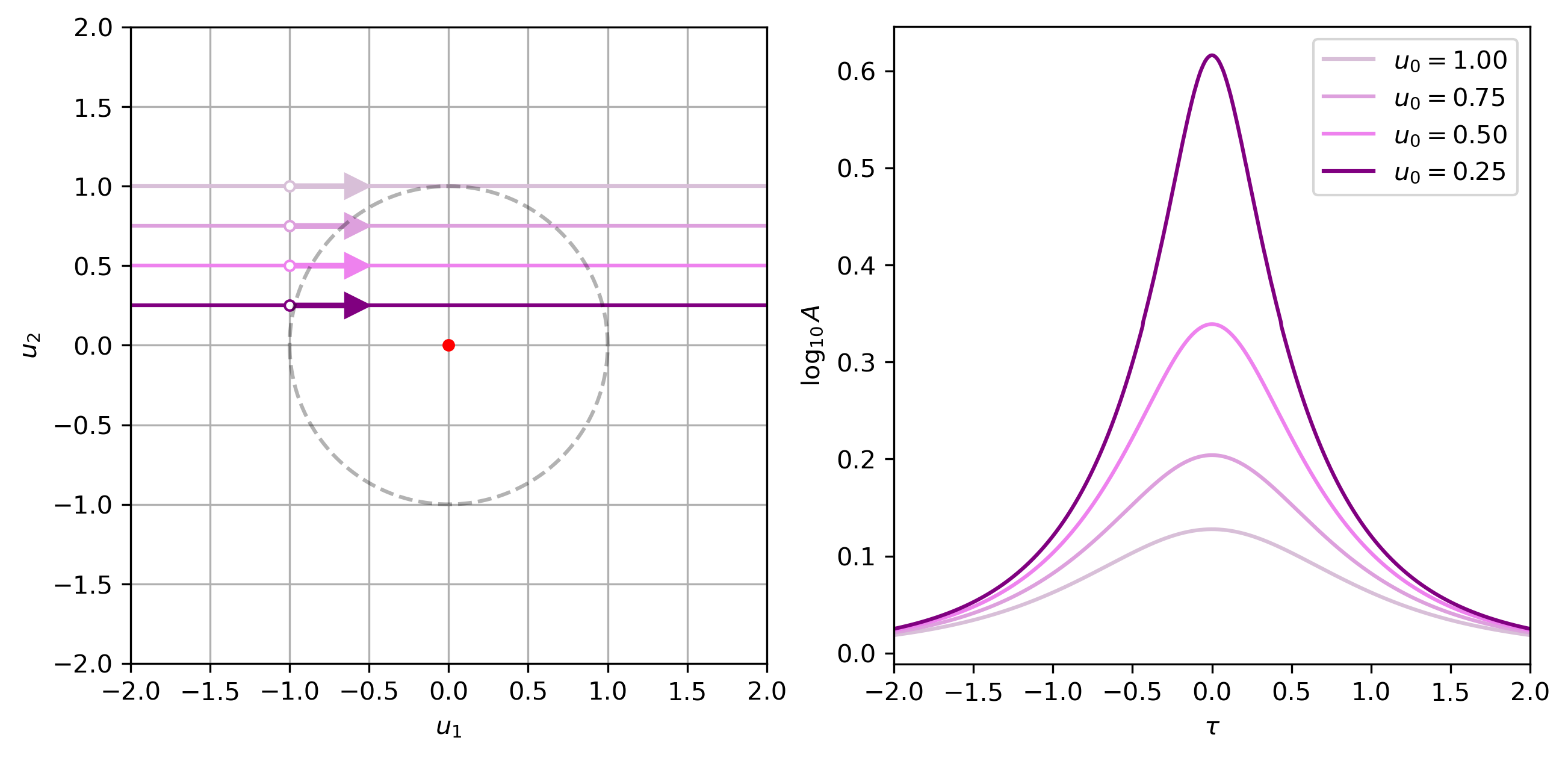
A larger \(u_0\) means a lower \(A_{\rm peak}\) and larger \(\rho\) means the magnification curve is more smoothed. This smoothing is termed the "finite-source effect." Theoretically, for a point source (\(\rho=0\)), \(A_{\rm peak}=\infty\) if \(u_0=0\). The basic shape of the lightcurves of these point-source-like events is referred to as a Paczynski curve.
If none of that sunk in, don't worry. You'll start to get a feel for it as we move through some examples. We will also learn how to make a figure like the one shown above in the notebook SingleLens.ipynb.
The slider below allows you to change the physical parameters of a lensing "event" to see how these changes in physical parameters affect the size of the Einstein ring. You may need to ensure the interactive plot's cell was the last code cell you ran, for the sliders to be active.
For quick conversions, it is worth noting that the Sun is about 1000 times the mass of Jupiter. So the mass of Jupiter is like one milli-solar masses. The duterium fusion limit is at about 10 Jupiter masses or 0.01 solar masses. The hydrogen fusion limit is around 100 Jupiter masses or 0.1 solar masses.
# Interactive Angular Eistein Ring Radius Plot

# If the plot does not present correctly in the notebook, try rerunning the cell.

theta_E_max = 5.5  # Maximum value for theta_E

%matplotlib widget

# Create the figure and axis globally so they are not recreated each time
plt.close(1)  # Close the previous figure if it exists
fig, ax = plt.subplots(num=1, figsize=(6, 6))

# Set plot background and text colors
ax.set_facecolor('black')
ax.spines['bottom'].set_color('white')
ax.spines['top'].set_color('white')
ax.spines['right'].set_color('white')
ax.spines['left'].set_color('white')
ax.tick_params(axis='x', colors='white')
ax.tick_params(axis='y', colors='white')

# Update the plot without making a new figure
fig.canvas.draw()

def update_plot(M: float, Dl: float, Ds: float) -> None:
    """
    Update the plot with the given lensing system parameters.

    Parameters
    ----------
    M : float
        Mass of the lens in solar masses
    Dl : float
        Distance to the lens in kpc
    Ds : float
        Distance to the source in kpc
    """

    global theta_E_max  # Use the global variable for the maximum theta_E value
    theta_E_value = theta_E(M, Dl, Ds)  # mas
    r_E_au = theta_E_value * Dl  # au
    pi_rel = 1.0/(Dl)-1.0/(Ds)  # mas  # CHECK THIS!
    r_E_au = Dl * theta_E_value  # au
    kappa = 8.144  # mas/M_Sun
    pi_E = theta_E_value / (kappa * M)  # mas

    # Update the maximum value if needed
    if theta_E_value > theta_E_max:
        theta_E_max = theta_E_value*1.1  # Increase the maximum value if needed

    # Clear the previous plot content but keep the figure and axis
    ax.cla()  # Clear only the current axes

    fig.patch.set_facecolor('black')  # Set the figure background color to black

    # Plot the circles  # ADD PIE!
    circle = Circle((0, 0), theta_E(M, Dl, Ds), edgecolor='white', facecolor='none', alpha=1.0,
                    label=r'$\theta_E=$%3.3f mas; $r_E=$%3.3f au; $\pi_{rel}=$%3.3f mas; $\pi_E=$%3.3f mas' %(theta_E_value, r_E_au, pi_rel, pi_E))
    ax.add_patch(circle)

    # hydrogen fusing mass-radius relation (0.1 < M < 1)
    R = M**0.8 / 0.57
    R_sun2au = 0.00465  # 1 R_sun = 0.00465 au
    rho_L = R * R_sun2au / Dl # kpc, au, -> mas

    # Plot an EXAGGERATED star to represent the lens
    bigger = 10
    star = Circle((0, 0), bigger * rho_L, edgecolor='yellow', facecolor='white')
    ax.add_patch(star)
    np.save('./Exercises/IntroductionE1.npy', bigger)

    # Set text colot to white
    ax.yaxis.label.set_color('white')
    ax.xaxis.label.set_color('white')
    ax.title.set_color('white')

    # Set labels and title
    ax.set_xlabel(r'$u_1$ (mas)')
    ax.set_ylabel(r'$u_2$ (mas)')
    ax.set_title('Einstein Ring Size')

    # Add a white grid
    ax.grid(True, color='darkgrey', alpha=0.5)

    # Set axis to be equal
    ax.set_aspect('equal', adjustable='box')

    # Set the limits to a fixed range for simplicity
    ax.set_xlim(-theta_E_max, theta_E_max)
    ax.set_ylim(-theta_E_max, theta_E_max)

    # Add a legend
    ax.legend(loc='upper right', facecolor='black', edgecolor='white', labelcolor='white')

    # Update the plot without making a new figure
    fig.canvas.draw()

# Function to update the Ds slider's minimum value based on Dl
def update_Ds_slider(*args):
    Ds_slider.min = Dl_slider.value + 0.1  # Ensure Ds > Dl, but too close will do silly stuff
    if Ds_slider.value <= Ds_slider.min:
        Ds_slider.value = Ds_slider.min

# Function to handle updates when sliders change
def update_sliders(change):
    # Pass the current values of M, Dl, and Ds to the plot update function
    update_plot(M_slider.value, Dl_slider.value, Ds_slider.value)

# Create interactive sliders and text boxes for M, Dl, and Ds
slider_style = {'description_width': '150px'}  # Set the width of the description textboxes
slider_layout = widgets.Layout(width='500px')  # Set the width of the slider bars

# Create interactive sliders and text boxes for M, Dl, and Ds
M_slider = widgets.FloatSlider(value=1.0, min=0.01, max=10.0, step=0.1,
                               description='Mass (solar masses)',
                               style=slider_style, layout=slider_layout)
M_text = widgets.FloatText(value=1.0)

Dl_slider = widgets.FloatSlider(value=4.0, min=1.0, max=10.0, step=0.1,
                                description='Lens Distance (kpc)',
                                style=slider_style, layout=slider_layout)
Dl_text = widgets.FloatText(value=4.0)

Ds_slider = widgets.FloatSlider(value=8.0, min=5.1, max=10.0, step=0.1,
                                description='Source Distance (kpc)',
                                style=slider_style, layout=slider_layout)
Ds_text = widgets.FloatText(value=8.0)

# Link sliders and text boxes
widgets.jslink((M_slider, 'value'), (M_text, 'value'))
widgets.jslink((Dl_slider, 'value'), (Dl_text, 'value'))
widgets.jslink((Ds_slider, 'value'), (Ds_text, 'value'))

# Update the Ds slider's minimum value when Dl changes
Dl_slider.observe(update_Ds_slider, 'value')

# Observe slider value changes to trigger plot updates
M_slider.observe(update_sliders, 'value')
Dl_slider.observe(update_sliders, 'value')
Ds_slider.observe(update_sliders, 'value')

# Display sliders and text boxes
display(widgets.HBox([M_slider, M_text]))
display(widgets.HBox([Dl_slider, Dl_text]))
display(widgets.HBox([Ds_slider, Ds_text]))

# Initial plot
update_plot(M_slider.value, Dl_slider.value, Ds_slider.value)
If these plots are still not workig for you, check your version in the cell below match those in the YAML.
import sys
import ipympl
import matplotlib
import numpy

print("Python version:", sys.version)
print("ipympl version:", ipympl.__version__)
print("matplotlib version:", matplotlib.__version__)
print("numpy version:", numpy.__version__)
Python version: 3.11.15 (main, Jun 16 2026, 21:41:52) [GCC 13.3.0]
ipympl version: 0.10.0
matplotlib version: 3.11.1
numpy version: 2.4.6
We are going to tackle our first exercie now. As a reminder, the model solutions for these exercises are in the
Exercisessubfolder. Also, you can visit the Progress Checklist to track you progress through the exercises in each notebook.
Exercise 1
If you went through the code for this plot, you may have noticed that the size of the lens star has been exaggerated. By what factor is the display star's angular radius too big?
Write you answer in the cell below.
answer = 0  # replace this value with your answer

if answer == np.load('./Exercises/IntroductionE1.npy'):
    print('Correct!')
else:
    print('Not quite. Try again.')
Not quite. Try again.
The plot below gives us an intuition for the scale of this angular Einstein radius in both the lens plane and projected onto the source plane.
# interactive Einstein radius plot; angular, physical, and projected into the lens plane.

theta_E_max = 5.0  # Maximum value for theta_E

%matplotlib widget

# Create the figure and axis globally so they are not recreated each time
plt.close(100)  # Close the previous figure, if it exists
fig, (ax1, ax2) = plt.subplots(2, 1, figsize=(6, 6), num=100)

fig.patch.set_facecolor('black')  # Set the figure background color to black

# Main plot: Einstein ring
#--------------------------

# Set plot background and text colors
ax1.set_facecolor('black')
ax1.spines['bottom'].set_color('white')
ax1.spines['top'].set_color('white')
ax1.spines['right'].set_color('white')
ax1.spines['left'].set_color('white')
ax1.tick_params(axis='x', colors='white')
ax1.tick_params(axis='y', colors='white')
ax1.yaxis.label.set_color('white')
ax1.xaxis.label.set_color('white')
ax1.title.set_color('white')

# Add a white grid
ax1.grid(True, color='darkgrey', alpha=0.5)

# Set axis to be equal
ax1.set_aspect('equal', adjustable='box')

# Secondary plot: Distance vs. Radius
#------------------------------------

# Set plot background and text colors
ax2.set_facecolor('black')
ax2.spines['bottom'].set_color('white')
ax2.spines['top'].set_color('white')
ax2.spines['right'].set_color('white')
ax2.spines['left'].set_color('white')
ax2.tick_params(axis='x', colors='white')
ax2.tick_params(axis='y', colors='white')
ax2.yaxis.label.set_color('white')
ax2.xaxis.label.set_color('white')

# Add a white grid
ax2.grid(True, color='darkgrey', alpha=0.5)

# Set axis limits
ax2.set_xlim(0, 10)
ax2.set_ylim(-30,  30)
ratio = 5/60  # Full height half width of plot axis 2

ax2.set_xlabel('test label')

# Update the plot without making a new figure
fig.canvas.draw()

def update_plot(M, Dl, Ds):

    global theta_E_max  # Use the global variable for the maximum theta_E value
    theta_E_value = theta_E(M, Dl, Ds)  # mas
    pi_rel = 1.0/(Dl)-1.0/(Ds)  # mas  # CHECK THIS!
    r_E_au = Dl * theta_E_value  # au
    kappa = 8.144  # mas/M_Sun
    pi_E = theta_E_value / (kappa * M)  # mas

    # Update the maximum value if needed
    if theta_E_value > theta_E_max:
        theta_E_max = theta_E_value*1.1  # Increase the maximum value if needed

    # Clear the previous plot content but keep the figure and axis
    ax1.cla()  # Clear only the current axes
    ax2.cla()  # Clear only the current axes

    # Main plot: Einstein ring
    #--------------------------

    ax1.yaxis.label.set_color('white')
    ax1.xaxis.label.set_color('white')
    ax1.title.set_color('white')

    # Plot the circles
    circle = Circle((0, 0), theta_E(M, Dl, Ds), edgecolor='white', facecolor='none',
                    alpha=1.0, label=r'$\theta_E=$%3.3f mas' %theta_E_value)
    ax1.add_patch(circle)

    # hydrogen fusing mass-radius relation (0.1 < M < 1)
    R = M**0.8 / 0.57
    R_sun2au = 0.00465  # 1 R_sun = ... au
    rho_L = R * R_sun2au / Dl # kpc, au, -> mas

    # Plot an EXAGGERATED star to represent the lens
    bigger = np.load('./Exercises/IntroductionE1.npy')
    star = Circle((0, 0), bigger * rho_L, edgecolor='yellow', facecolor='white')
    ax1.add_patch(star)

    # Set the limits to a fixed range for simplicity
    ax1.set_xlim(-theta_E_max, theta_E_max)
    ax1.set_ylim(-theta_E_max, theta_E_max)

    # Add a legend
    ax1.legend(loc='upper right', facecolor='black', edgecolor='white', labelcolor='white')

    # Add a white grid
    ax1.grid(True, color='darkgrey', alpha=0.5)

    # Set labels and title
    ax1.set_xlabel(r'$u_1$ (mas)')
    ax1.set_ylabel(r'$u_2$ (mas)')
    ax1.set_title('Einstein Ring Size')

    # Secondary plot: Distance vs. Radius
    #------------------------------------

    ax2.yaxis.label.set_color('white')
    ax2.xaxis.label.set_color('white')

    # Plot the lens star
    R_au = R * R_sun2au
    lens_star = Ellipse((Dl, 0), width=(bigger * R_au * 2 * ratio), height=(bigger * R_au * 2),
                        edgecolor='yellow', facecolor='white')
    lens_star.set_zorder(1)
    ax2.add_patch(lens_star)
    Earth = Ellipse((0, 0), width=(ratio), height=1, edgecolor='green', facecolor='blue')
    Earth.set_zorder(1)
    ax2.add_patch(Earth)
    Source = Ellipse((Ds, 0), width=(ratio), height=1, edgecolor='red', facecolor='yellow')
    Source.set_zorder(1)
    ax2.add_patch(Source)

    # Plot the Einstein ring as an ellipse
    einstein_ring = Ellipse((Dl, 0), width=0.1, height=2 * r_E_au, edgecolor='white',
                            facecolor='none', alpha=1.0,
                            label=r'$r_E=$%3.3f au; $\pi_{rel}=$%3.3f mas; $\pi_E=$%3.3f mas' %(r_E_au, pi_rel, pi_E))
    ax2.add_patch(einstein_ring)

    # Projected ojnto the source plane
    einstein_ring_proj = Ellipse((Ds, 0), width=(0.1 * Ds / Dl), height=2 * Ds * theta_E_value,
                                 edgecolor='white', facecolor='none', linestyle='dotted', alpha=0.8)
    ax2.add_patch(einstein_ring_proj)

    # Plot the projection lines
    ax2.plot([0, 10], [0, 0], color='white', linestyle='-', zorder=0, linewidth=0.5)
    ax2.plot([0, Ds], [0, Ds * theta_E_value], color='white', linestyle='--', zorder=0, linewidth=0.5)
    ax2.plot([0, Ds], [0, -Ds * theta_E_value], color='white', linestyle='--', zorder=0, linewidth=0.5)

    # Add a white grid
    ax2.grid(True, color='darkgrey', alpha=0.5)

    # Set axis limits
    ax2.set_xlim(0, 10)
    ax2.set_ylim(-30,  30)

    # Set labels and title
    ax2.set_xlabel('Distance (kpc)')
    ax2.set_ylabel('Radius (au)')

    # Add a legend
    ax2.legend(loc='upper right', facecolor='black', edgecolor='white', labelcolor='white')

    # Update the plot without making a new figure
    fig.canvas.draw()

def update_Ds_slider(*args):
    Ds_slider.min = Dl_slider.value + 0.1  # Ensure Ds > Dl, but too close will do silly stuff
    if Ds_slider.value <= Ds_slider.min:
        Ds_slider.value = Ds_slider.min

# Function to handle updates when sliders change
def update_sliders(change):
    # Pass the current values of M, Dl, and Ds to the plot update function
    update_plot(M_slider.value, Dl_slider.value, Ds_slider.value)

# Create interactive sliders and text boxes for M, Dl, and Ds
slider_style = {'description_width': '150px'}  # Set the width of the description textboxes
slider_layout = widgets.Layout(width='500px')  # Set the width of the slider bars

M_slider = widgets.FloatSlider(value=1.0, min=0.01, max=10.0, step=0.1,
                               description='Mass (solar masses)',
                               style=slider_style, layout=slider_layout)
M_text = widgets.FloatText(value=1.0)

Dl_slider = widgets.FloatSlider(value=4.0, min=0.5, max=10.0, step=0.1,
                                description='Lens Distance (kpc)',
                                style=slider_style, layout=slider_layout)
Dl_text = widgets.FloatText(value=4.0)

Ds_slider = widgets.FloatSlider(value=8.0, min=5.1, max=10.0, step=0.1,
                                description='Source Distance (kpc)',
                                style=slider_style, layout=slider_layout)
Ds_text = widgets.FloatText(value=8.0)

# Link sliders and text boxes
widgets.jslink((M_slider, 'value'), (M_text, 'value'))
widgets.jslink((Dl_slider, 'value'), (Dl_text, 'value'))
widgets.jslink((Ds_slider, 'value'), (Ds_text, 'value'))

# Update the Ds slider's minimum value when Dl changes
Dl_slider.observe(update_Ds_slider, 'value')

# Observe slider value changes to trigger plot updates
M_slider.observe(update_sliders, 'value')
Dl_slider.observe(update_sliders, 'value')
Ds_slider.observe(update_sliders, 'value')

# Display sliders and text boxes
display(widgets.HBox([M_slider, M_text]))
display(widgets.HBox([Dl_slider, Dl_text]))
display(widgets.HBox([Ds_slider, Ds_text]))

# Initial plot
update_plot(M_slider.value, Dl_slider.value, Ds_slider.value)
You might also note how, for a given lens distance, the angular Einstein radius is at its smallest when the source-lens distance (\(D_S-D_L\)) is small. Objects in the same system, such as binary stars, would have extremely small Einstein rings and therefore a very large fninite source effect, which is why we don't see events of this kind. However, larger source-lens distances have diminishing returns in terms of the increase in angular Einstein radius. To demonstrate, we have made a plot of \(\theta_E\) vs \(D_S-D_L\). The line on this plot represents a fixed \(M_L\) and \(D_L\) (1 \(M_\odot\), 1 kpc).
Note. You can navigate to the sample solutions quickly but clicking on the exercise title, e,g, "Exercise 2" (you may need to allow the pop-up).
colours = ['red', 'green', 'blue', 'orange']

M = 1.0  # M_sun
Dl = 1.0  # kpc
Ds = np.linspace(Dl, 10, 100)  # kpc
Ds = Ds[1:]  # Remove Ds = Dl

theta_E_values = np.array([theta_E(M, Dl, D) for D in Ds])

plt.close(2)  # Close the previous figure, if it exists
plt.figure(num=2, figsize=(8, 5))  # Create a new figure
plt.plot(Ds, theta_E_values, color=colours[0], label=r'$M_L=1.000M_\odot$, $D_L=1$ kpc')

######################
# EXERCISE: IntroductionE2.txt
#---------------------
# Your code goes here

######################

plt.xlabel(r'Source Distance, $D_{\rm{S}}$ (kpc)')
plt.ylabel(r'Angular Einstein Radius, $\theta_{\rm{E}}$ (mas)')
plt.legend(loc='lower left', ncol=3, fontsize='small')
plt.show()
Exercise 3
For a fixed mass and source distance, the Einstein radius (rE) peaks at DL=DS/2. Make a plot of rE vs DL for a fixed ML and DS.
plt.close(3)
plt.figure(num=3, figsize=(9, 5))

######################
# EXERCISE: IntroductionE3.txt
#---------------------
# Your code goes here

######################

plt.show()
If you are wondering why all of the distances have been restricted to between 0 and 10 kpc, this will become clear once you have completed Galactic Models (in preperation) and the Optical Depth section in Simulations (in preperation). Put simply, the Galactic center is at about 8 kpc from the Sun and the density of stars is much greater there than it is closer to the Sun. There is another effect that affects plausible source distances and that is the extinction in the field.
Current, ground-based*3 observing strategies concentrate on fields close to the Galactic center to maximise the number of stars that are visible and therefore the return of observed microlensing events. However, these fields are also impeded by dust from the plane of the Galactic disk. The result is that, ground-based, I- and V-band surveys, do not observe source stars much more distant than the Galactic center, because the extinction in these bands, with these pointings, is too high.
*3 Ground-based observing strategies, as of 2025.
2. What is it used for?#
Because only the source light is magnified in a microlensing event, the luminosity of the lens system does not directly contribute to the event's detectability. As a result, microlensing is uniquely capable when it comes to detecting cold, low-mass, dim lenses, such as brown dwarfs and unbound planetary-mass objects, or massive dark lenses like black holes. Additionallly, it has unique sensitivities in the detection of bound planets outside our solar system (exoplanets).
In the case where multiple bound objects make up the lens, the resulting magnification will manifest in a manner related to the event's geometry and the mass ratio of the lens system. This means that secondary (companion) objects in bound orbits around the primary (host) objects within the lens, which may or may not be dim, can also be uncovered. Lenses made up of more than one lens object have more complicated geometries with projected source positions of theoretical infinite magnification (given a point source) called caustic curves, and images that form around critical curves, like the undulating bright lines you see when light passes through turbulent water. A more detailed description of critical and caustic curves and model parameterisations is given in the Binary Lens notebook (in development). Events with one source and two lens bodies are referred to as binary lens events. These are the events that typically result in microlensing bound-planet detections.
We continue to introduce exoplanet detection, free-floating planets and brown dwarf in details in the Planets. We also cover black holes and other remnants, and microlensing's ties to dark matter in the Remnants and Dark Matter notebook.
Next steps#
You finished your first notebook. Good job! if the Python was a bit much, you can always skip those exercises by copying in the sample answer from the Exercises folder. If you would like to continue doing the Python exercises, but need to take a step back and brush up on your skills, try checking out the Carpentries Incubator course.
The next notebook you should try is:
But these would also be good choices:
Photometry (in development)
The Galactic Model (in preparation)
NGRST (in preparation)
If none of those tickle you fancy, try picking any one of the other notebooks within the Notebooks directory. The top of each notebook will tell you if there are any other notebooks that are recommended to be completed before starting, but this is your journey; you do you.