This is a brief notebook, but it is heavily reliant on the concepts covered in the Single Lens notebook. If you have not completed that notebook, perhaps it would be best if you did that and then came back.
If you haven't already done so, install MulensModel before continuing with this notebook:
pip install MulensModel
# package imports (SHIFT + ENTER to run)
import numpy as np
import emcee
import MulensModel as mm
import matplotlib.pyplot as plt
import multiprocessing as mp
from IPython.display import display, clear_output
from typing import List, Tuple, Optional, Union

# dev note: replace emcee with dynesty?
The binary source model#
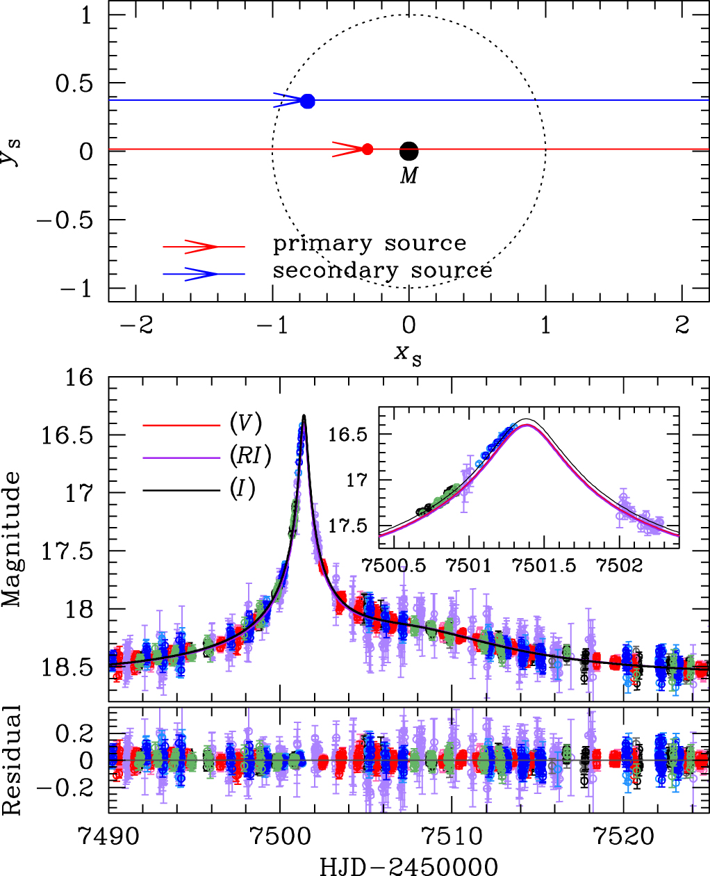
Events matching a one-lens, two-sources model typically have lightcurves with smooth non-Paczynski shapes, such as the one in Jung et al. (2017), Figure 5, which is shown below (event OGLE-2016-BLG-0733). They are, in effect, two distinct Paczynski curves on top of each other; they do not create "sharp" perturbations from the primary Paczynski curve, like the binary-lens models typically do.
|
|
|---|---|
[Reproduction of Jung et al. (2017), Figure 5] Geometry and lightcurve of the binary-source model. Top: The upper panel shows the geometry of the binary-source model. Two straight lines with arrows are the source trajectories of individual source stars. The lens is located at the origin (marked by M), and the dotted circle is the angular Einstein ring. The red and blue filled circles represent the individual source positions at \(\rm{HJD}'=7497\). Lengths are normalised by the Einstein radius. Bottom: The lower panel shows the enlarged view of the anomaly region. The two curves with different colours are best-fit binary-source models for \(RI\) and \(I\) passbands. The inset shows a zoom of the anomaly near \(\rm{HJD}'\sim7501.4\). We note that, although we only use the \(V\)-band data for determining the source type, we also present the \(V\)-band model lightcurve to compare the colour change between passbands. |
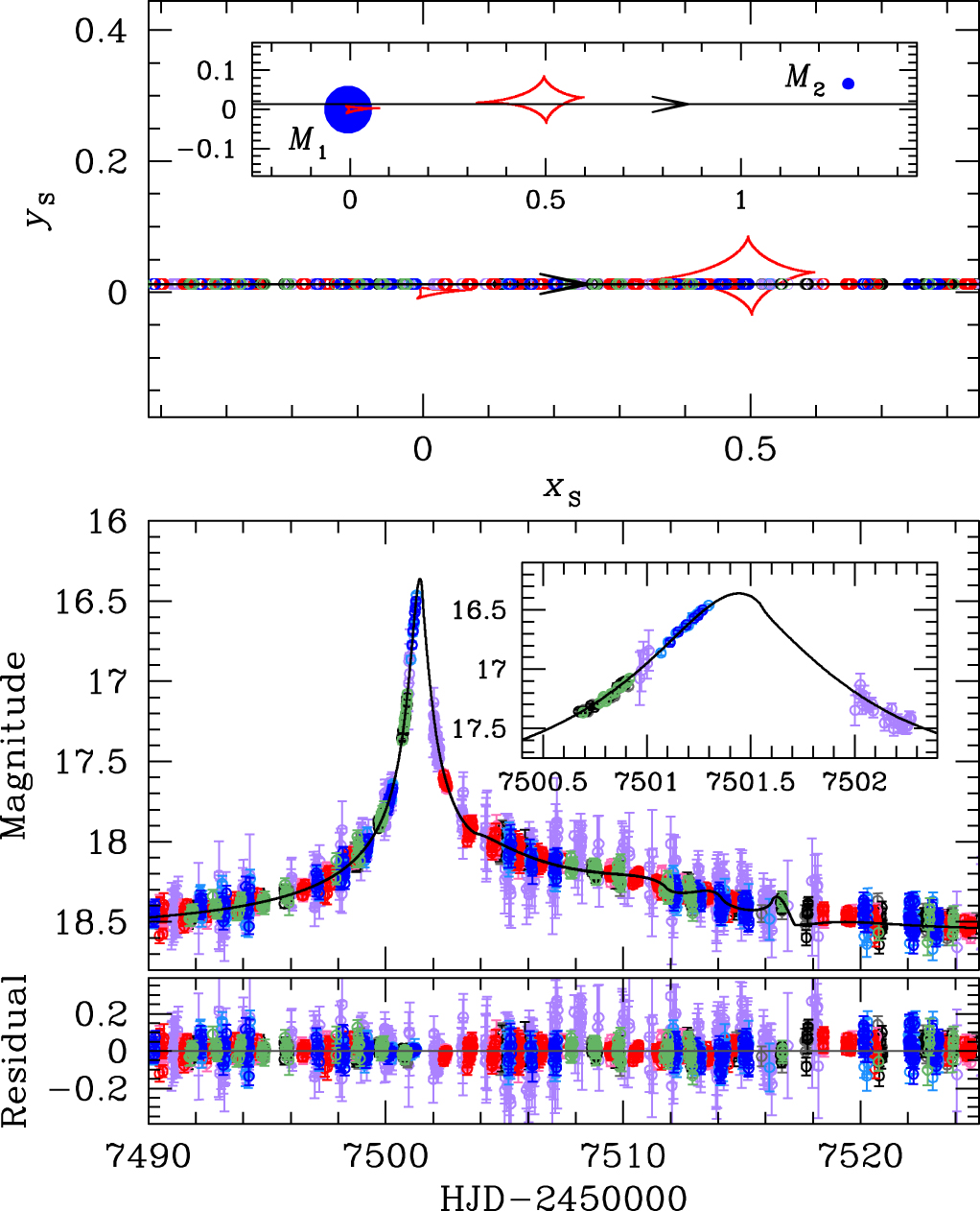
[Reproduction of Jung et al. (2017), Figure 3] Geometry and lightcurve of the binary lens model. Top: The upper panel shows the geometry of the binary lens model. The straight line with an arrow is the source trajectory, red closed concave curves represent the caustics, and blue filled circles (marked by \(M_1\) and \(M_2\)) are the binary lens components. All length scales are normalised by the Einstein radius. The inset shows the general view and the major panel shows the enlarged view corresponding to the lightcurve of the lower panel. The open circle on the source trajectory is the source position at the time of observation whose size represents the source size. Bottom: The lower panel shows the enlarged view of the anomaly region. The inset shows a zoom of the lightcurve near \(\rm{HJD}'\sim7501.4\). The curve superposed on the data is the best-fit binary lens model. |
The magnification model has the same parameterisation as the single lens model, except the flux model is a sum of two single-source magnifications multiplied by the flux of the source they are lensing:
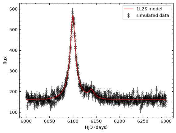
We can see the model in practice in the code cell below:
# A simulated binary source event

t01, u01 = 6100., 0.2  # primary source model parameters
t02, u02 = 6140., 0.2  # secondary source model parameters
t_E = 25.   # tE is not necessarily the same, due to orbital motion of the lens system, but we would expect
            # tE to be mostly due to the relative propermotion of the lens and source systems.
flux1, flux_ratio, blend_flux = 100., 0.1, 50.
n = 500  # number of data points
time = np.linspace(6000., 6300., n)  # "data" epochs
N = 1000  # model plotting precision
T = np.linspace(6000., 6300., N)  # model time array

# building the individual magnification models for each source star
model1 = mm.Model({'t_0': t01, 'u_0': u01, 't_E': t_E})
A1 = model1.get_magnification(time)
model2 = mm.Model({'t_0': t02, 'u_0': u02, 't_E': t_E})
A2 = model2.get_magnification(time)

flux = A1 * flux1 + A2 * flux1*flux_ratio + blend_flux
flux_err = 3.0 *(np.abs(5.0 + np.random.normal(size=n)))  # flux uncertainties with mu=15 and std=3
error = flux_err * np.random.normal(size=n)     # offset the "meaasurments" by an amount that is dependent
flux += error                                   # on the uncertainty
data = [time, flux, flux_err]

my_dataset = mm.MulensData(data, phot_fmt='flux')

plt.close(1)
plt.figure(1)

# Plot the data
plt.errorbar(time, flux, yerr=flux_err,
             fmt='x',
             ecolor='k',
             capsize=1,
             color='k',
             alpha=0.6,
             zorder=0,
             label='simulated data'
             )
# Plot the model
F = model1.get_magnification(T) * flux1 + model2.get_magnification(T) * flux1*flux_ratio + blend_flux
plt.plot(T, F,
         color='r',
         linestyle='-',
         lw=1,
         zorder=1,
         label='1L2S model'
         )

plt.legend()
plt.xlabel(r'HJD (days)')
plt.ylabel(r'flux')
plt.show()
The measure of how far the data are from the model solution, scaled by the data uncertainties (\(\chi^2\)), is calculated using
Similar to the procedure in the Single Lens notebook, the maximum likelihood solution \((F_{\rm S1}, F_{\rm S2}, F_{\rm B})\) can therefore be found by solving for the minima of this function. As in the previous section, the minima occurs where the partial derivatives of the \(\chi^2\) function are 0;
which is solved following as follows:
Exercise 1
Use linear regression to determine the flux of the primary source, secondary source, and blend stars. Did you get out something similar to what you put in?
You may want to consider using functions from the numpy.linalg module.
# objective function
def binary_source_chi2(theta: np.ndarray,
                       model1: mm.Model,
                       model2: mm.Model,
                       data: List,
                       verbose: Optional[bool] = False,
                       return_fluxes: Optional[bool] = False
                       ) -> float:
    """
    chi2 function for a binary-source, single-lens, microlensing model.

    Parameters
    ----------
    theta : np.ndarray
        Array of model parameters being fit.
    model1 : mm.Model
        Primary source model.
    model2 : mm.Model
        Secondary source model.
    data : list
        List of data arrays.
    verbose : bool, optional
        Default is False.
        Print the primary source flux, secondary source flux, and blend flux.

    Returns
    -------
    float
        The chi2 value.

    Notes
    -----
    The model parameters are unpacked from theta and set to the model1 and model2 parameters.
    model1 and model2 are MulensModel.Model objects; see MulensModel documentation
    (https://rpoleski.github.io/MulensModel/) for more information.
    """
    #unpack the data
    t, flux, flux_err = data

    # model parameters being fit
    labels = ['t_0', 'u_0', 't_E']

    # change the values of model.parameters to those in theta.
    theta1 = theta[:3]
    theta2 = theta[3:]
    for (label, value1, value2) in zip(labels, theta1, theta2):
        setattr(model1.parameters, label, value1)
        setattr(model2.parameters, label, value2)

    # calculate the model magnification for each source
    A1 = model1.get_magnification(t)
    A2 = model2.get_magnification(t)

    ######################
    # EXERCISE: BinarySourceE1.txt
    #---------------------
    # build the matricies for the linear algebra
    C = np.array([np.sum(A1 * flux * flux_err**-2), np.sum(A2 * flux * flux_err**-2), np.sum(flux * flux_err**-2)])
    B = np.array([[np.sum(A1**2 * flux_err**-2), np.sum(A1 * A2 * flux_err**-2), np.sum(A1 * flux_err**-2)],
                  [np.sum(A1 * A2 * flux_err**-2), np.sum(A2**2 * flux_err**-2), np.sum(A2 * flux_err**-2)],
                  [np.sum(A1 * flux_err**-2), np.sum(A2 * flux_err**-2), np.sum(flux_err**-2)]])

    # calculate the flux components
    Theta = np.linalg.solve(B, C)  # ax=b <- B x Theta = C
    FS1, FS2, FB = Theta # primary source flux, secondary source flux, and blend flux
    ######################

    # print the flux parameters
    if verbose:
        print(f"Primary source flux: {FS1}")
        print(f"Secondary source flux: {FS2}")
        print(f"Blend flux: {FB}")

    # calculate the model flux
    model_flux = A1 * FS1 + A2 * FS2 + FB
    chi2 = np.sum(((flux - model_flux) / flux_err)**2)

    # In case something goes wrong with the linear algebra
    if np.isnan(chi2) or np.isinf(chi2):
        print(f"NaN or inf encountered in chi2 calculation: theta={theta}, chi2={chi2}")
        return 1e16

    if return_fluxes:
        return chi2, FS1, FS2, FB
    else:
        return chi2


# generative model parameters
t01, u01 = 6100., 0.2
t02, u02 = 6140., 0.2
t_E = 25.
theta = np.array([t01, u01, t_E, t02, u02, t_E])

# initial chi2 value (will print the fluxes)
chi2 = binary_source_chi2(theta, model1, model2, data, verbose=True)

# generative fluxes
# source 2 flux used to generate the data
flux2 = flux1 * flux_ratio
print('\nprimary source flux used to generate the data:', flux1)
print('secondary source flux used to generate the data:', flux2)
print('blend flux used to generate the data:', blend_flux)
Primary source flux: 99.72628370195058
Secondary source flux: 10.67581685379159
Blend flux: 49.45049580932277

primary source flux used to generate the data: 100.0
secondary source flux used to generate the data: 10.0
blend flux used to generate the data: 50.0
The noise we generated in the light curve should mean that, even though we used the "true" magnification-model parameters, the flux values we retrieve are not exactly the same as those we used to generate the lightcurve. But they should be close (i.e. within a few flux units). If you got values that are wildly different something has gone wrong. It could be a fluke, so start be regenerating your noisy data. If that doesn't fix the problem you will need to take another look at your \(\chi^2\) function (Exercise 1).
Exercise 2
Make an initial guess at the parameters for this model.
I know, we know them. Pretend we don't, okay.
######################
# EXERCISE: BinarySourceE2.txt
#---------------------
# initial guess
t01 = 6100
t02 = 6140
u01 = 0.2
u02 = 0.3
tE1 = 25
tE2 = 25

# fitting the model
theta0 = [t01, u01, tE1, t02, u02, tE2]
######################
Next we are going to try fitting the data. Even though the likelihood space for a binary-source model should be reasonably well behaved, we will fit this simulated event using MCMC (emcee), because we want to take a look at the posteriors from the fit, so that we can understand if there are any degeneracies between magnification-model parameters. We can use emcee to both fit and collect our posterior samples.
If that all sounded like a forgein language to you, you might need to check-out, or revist, the Modelling notebook.
Exercise 3
Apply some reasonable bounds on the magnification-model parameters (theta).
Replace "True" with your conditions for what constitutes unresonable model-parameter values.
def ln_prob(theta: np.ndarray, model1, model2, data) -> float:
    """log probability"""

    lp = 0.0

    ######################
    # EXERCISE: BinarySourceE3.txt
    #---------------------
    # priors                         # replace True with conditions

    # add a constraint on tEs with a 1 sig deltatE of 5 days
    lp += -(theta[2]-theta[5])**2/5**2   # this discourages the tEs from being too different

    if np.any(np.array(theta) < 0) or theta[0] > theta[3] or theta[0] < 6000 or theta[3] < 6000 or theta[0] > 6300 or theta[3] > 6300:
        return -1e16

    elif (theta[2]-theta[5])**2 > 20**2:  # max 20 days difference
        return -1e16
    ######################

    else: # the proposed parameters values are reasonable

        ######################
        # EXERCISE: BinarySourceE7.txt
        #---------------------
        #chi2 = binary_source_chi2(theta, model1, model2, data, return_fluxes=False)
        chi2, FS1, FS2, FB = binary_source_chi2(theta, model1, model2, data, return_fluxes=True)

        # implement a prior demanding positive fluxes
        if FS1 < 0 or FS2 < 0 or FB < 0:
            lp = -1e16
        ######################

        # return the log probability
        return -0.5 * chi2 + lp

# starting lnL
lnP = ln_prob(theta0, model1, model2, data)
print('initial log probability:', lnP)
initial log probability: -245.73703085948318
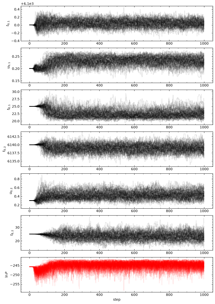
This model is pretty simple. It shouldn't take too long to converge; 1000 steps should be more than enough.
Exercise 4
Set up the emcee sample by choosing the fitting parameters you would like to use.
Note. there is only one correct value for ndim, but the other parameters are more nebulous.
# emcee parameters
nsteps = 1000
######################
# EXERCISE: BinarySourceE4.txt
#---------------------
nwalkers = 100
ndim = len(theta0)
steps_between_plot_updates = 100
######################

# Set up the sampler
sampler = emcee.EnsembleSampler(nwalkers, ndim, ln_prob,
                                args=[model1, model2, data])
Exercise 5
Create an initial state for you walkers.
Note. These should be "random" values, close to your initial guess; the walkers should start in a hyper-dimensional ball in parameter space, about the inital guess. You might want to consider the np.random.randn function.
######################
# EXERCISE: BinarySourceE5.txt
#---------------------
# Initialize the walkers
initial_pos = theta0 + 1e-6 * np.random.randn(nwalkers, ndim)
######################
# Function to update the plot
def update_plot(sampler, nwalkers, fig, axes):
    ylabels = [r'$t_{0,1}$', r'$u_{0,1}$', r'$t_{\rm{E},1}$',
               r'$t_{0,2}$', r'$u_{0,2}$', r'$t_{\rm{E},2}$',
               r'$\ln{P}$']
    for j in range(ndim):
        axes[j].clear()
        for i in range(nwalkers):
            axes[j].plot(sampler.chain[i, :, j], 'k', alpha=0.1)
        axes[j].set_ylabel(ylabels[j])

    axes[ndim].clear()
    for i in range(nwalkers):
        axes[ndim].plot(sampler.lnprobability[i], 'r', alpha=0.1)
    axes[ndim].set_ylabel(ylabels[ndim])
    axes[ndim].set_xlabel('step')

    clear_output(wait=True)
    display(fig)
    fig.canvas.draw()
    fig.canvas.flush_events()

def run_emcee(sampler: emcee.EnsembleSampler,
              initial_pos: np.ndarray,
              nsteps: int,
              steps_between_plot_updates: int,
              nwalkers: int,
              ndim: int,
              verbose: Optional[bool] = True
              ) -> Tuple[emcee.EnsembleSampler, np.ndarray]:
    """
    Run the emcee sampler and update the plot.

    Parameters
    ----------
    sampler : emcee.EnsembleSampler
        The sampler object.
    initial_pos : np.ndarray
        The initial position of the walkers.
    nsteps : int
        The number of steps to run the sampler.
    steps_between_plot_updates : int
        The number of steps between plot updates.
    nwalkers : int
        The number of walkers.
    ndim : int
        The number of dimensions.
    verbose : bool, optional
        Default is False.
        Print the progress of the sampler.
    """
    # Create the figure and axes
    fig, axes = plt.subplots(ndim + 1, 1, figsize=(10, 15));

    # Run the sampler in steps and update the plot
    i = 0
    while i < nsteps:
        if i == 0:
            state = sampler.run_mcmc(initial_pos, steps_between_plot_updates, progress=verbose)
        else:
            state = sampler.run_mcmc(state, steps_between_plot_updates, progress=verbose)
        update_plot(sampler, nwalkers, fig, axes)
        i += steps_between_plot_updates
    clear_output(wait=True)  # extra stuff to stop the notebook displaying the final plot twice

    # Access the final state
    final_state = sampler.get_last_sample().coords

    return sampler, final_state

# Run the sampler
sampler.reset() # reset the sampler (you will need this if you want to run_emee fresh, from initial_pos)
sampler, final_state = run_emcee(sampler, initial_pos, nsteps,
                                 steps_between_plot_updates, nwalkers, ndim)

# continue running  (use this if you want more steps after the first run)
#sampler, final_state = run_emcee(sampler, final_state, nsteps,
#                                 steps_between_plot_updates, nwalkers, ndim)
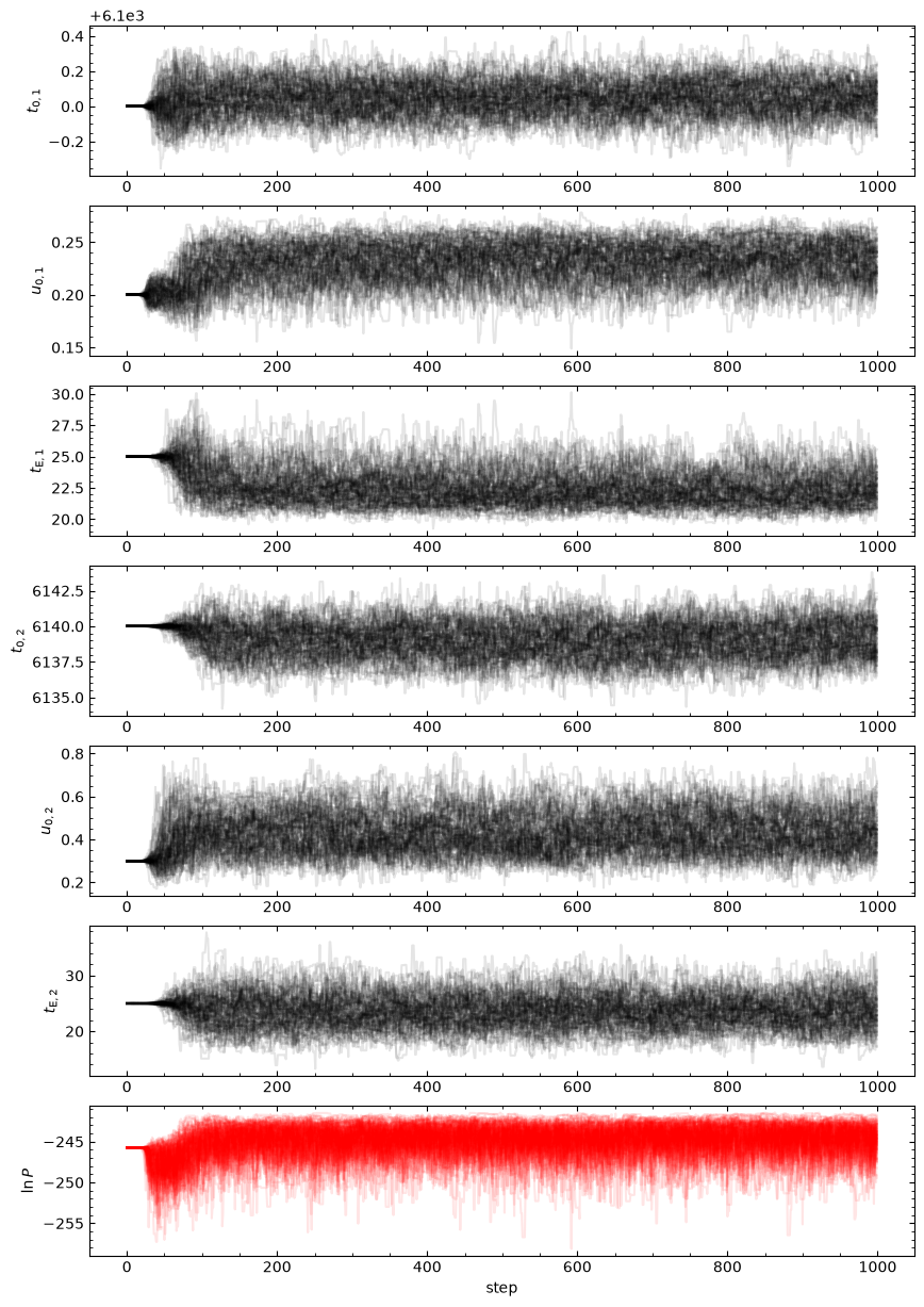
Depnding on the priors you chose and the random errors you generated, you may find that u02, tE2, or both are very poorly contrained; this would look like a large spread in the chains for those parameters. You could consider a prior that links the tE values to something similar to each other. But we may also decide to apply a prior constraint on the blend flux, which we reasonable know should not be negative for simulated data.
Why don't we take a look at the flux parameters for the final state and see if we can figure out what is going on?
# corner-like scatter plot of final state: u02, t02, FS2, FB
def plot_corner(final_state: np.ndarray,
                model1: mm.Model,
                model2: mm.Model,
                data: list,
                figure_number: Optional[int] = 3
                ) -> None:
    """
    Plot the corner-like scatter plot of the final state.

    Parameters
    ----------
    final_state : np.ndarray
        Array of final state parameters.
    model1 : mm.Model
        Primary source model.
    model2 : mm.Model
        Secondary source model.
    data : list
        List of data arrays.
    figure_number : int, optional
        Default is 3.
        The figure number.
    """
    # labels
    labels = [r'$t_{0,1}$', r'$u_{0,1}$', r'$t_{E,1}$', r'$t_{0,2}$', r'$u_{0,2}$', r'$t_{E,2}$', r'$F_{S,1}$', r'$F_{S,2}$', r'$F_B$']

    # collect the data dor plotting
    corner_array = np.zeros((len(final_state), ndim + 4))
    corner_array[:, 0:ndim] = final_state

    for i in range(len(final_state)):
        chi2, FS1, FS2, FB = binary_source_chi2(final_state[i], model1, model2, data, return_fluxes=True)
        corner_array[i,ndim] = FS1
        corner_array[i,ndim + 1] = FS2
        corner_array[i,ndim + 2] = FB
        corner_array[i,ndim + 3] = chi2

    # plot
    plt.close(figure_number)
    plt.figure(figure_number)
    fig, axes = plt.subplots(ndim + 3, ndim + 3, figsize=(15, 15))

    for i in range(ndim+3):
        for j in range(ndim+3):
            if i > j:  # plot the scatter plots
                scatter = axes[i, j].scatter(corner_array[:, j],
                                            corner_array[:, i],
                                            c=corner_array[:, -1],
                                            cmap='viridis_r',
                                            s=0.5
                                            )

                if i == ndim + 2:
                    axes[i, j].set_xlabel(labels[j])
                else: #turn of ticks labels
                    axes[i, j].set_xticks([])

                if j == 0:
                    axes[i, j].set_ylabel(labels[i])
                else: #turn of ticks labels
                    axes[i, j].set_yticks([])

            elif i == j:  # plot the histograms

                axes[i, j].hist(corner_array[:, j], bins=20, color='k')

                if i == ndim + 2:
                    axes[i, j].set_xlabel(labels[j])
                else:
                    axes[i, j].set_xticks([])

                axes[i, j].set_yticks([])

            else:  # turn off the upper triangle of axis
                axes[i,j].axis('off')


    # Add the colorbar using the scatter plot object
    cbar = fig.colorbar(scatter, orientation='horizontal', ax=axes, aspect=100)
    cbar.set_label('chi2')

    plt.show()

plot_corner(final_state, model1, model2, data)
<Figure size 640x480 with 0 Axes>
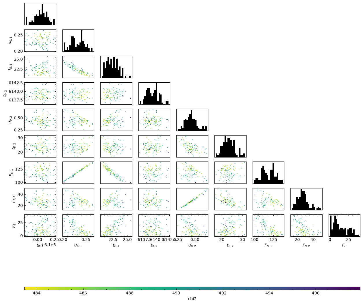
Do you see the problem? Negative blend-flux values are allowing for overly high \(F_{\rm{S},2}\) values, in combination with correspondong low \(t_{\rm{E},2}\) and high \(u_{0,2}\). We can avoid this problem by not allowing negative blending, which, considering our data was generated without using photometry, makes absolutely no sense. For events found in real data a small negative flux can be plausible as it is an indication that the "zero flux" background-level in the photometry was actually measuring some flux from stars. In these cases, the blend flux should actually have been measured as very small or 0.
Exercise 7
Add a prior on blend flux in ln_prob() function (Exercies 3) and any other additional priors you think seem reasonable.
######################
# EXERCISE: BinarySourceE8.txt PART: 1
#---------------------
# re make the sampler  (Make sure to run the ln_prob cell after you edit it)
sampler = emcee.EnsembleSampler(nwalkers, ndim, ln_prob,
                                args=[model1, model2, data])

# rerun the sampler
run_emcee(sampler, initial_pos, nsteps, steps_between_plot_updates, nwalkers, ndim)
######################
(<emcee.ensemble.EnsembleSampler at 0x7fe031b5bb90>,
 array([[6.09997911e+03, 2.04852100e-01, 2.40945638e+01, 6.13974579e+03,
         4.08619780e-01, 2.73065166e+01],
        [6.10000113e+03, 2.34052038e-01, 2.19842276e+01, 6.13881031e+03,
         4.62040509e-01, 2.16992861e+01],
        [6.10001594e+03, 2.33738348e-01, 2.26611878e+01, 6.13777859e+03,
         4.85596814e-01, 1.97616598e+01],
        [6.10012541e+03, 2.22276590e-01, 2.35775686e+01, 6.14174008e+03,
         4.80833111e-01, 1.95142663e+01],
        [6.10001515e+03, 2.24024583e-01, 2.24656666e+01, 6.13732159e+03,
         5.07537606e-01, 2.44562542e+01],
        [6.10021863e+03, 2.35018698e-01, 2.19532097e+01, 6.13977470e+03,
         5.20774477e-01, 1.94864263e+01],
        [6.09991028e+03, 2.34193140e-01, 2.21377368e+01, 6.14084796e+03,
         2.95064618e-01, 3.06243067e+01],
        [6.09998275e+03, 2.52003743e-01, 2.12193281e+01, 6.13838708e+03,
         3.80579662e-01, 2.71002641e+01],
        [6.10008710e+03, 2.14197262e-01, 2.42018158e+01, 6.13883619e+03,
         5.61201816e-01, 2.27075517e+01],
        [6.09996839e+03, 2.18571573e-01, 2.31230395e+01, 6.13876137e+03,
         5.78093033e-01, 2.38889022e+01],
        [6.10001195e+03, 2.49347511e-01, 2.13500674e+01, 6.13853747e+03,
         3.15164405e-01, 2.21346608e+01],
        [6.10020752e+03, 2.24627176e-01, 2.24301552e+01, 6.13902130e+03,
         5.87845602e-01, 2.05717874e+01],
        [6.10003980e+03, 2.19114027e-01, 2.27083243e+01, 6.13696412e+03,
         6.49713275e-01, 2.23214173e+01],
        [6.10009375e+03, 2.60006474e-01, 2.07502661e+01, 6.13888552e+03,
         3.25116567e-01, 2.88787891e+01],
        [6.09985756e+03, 2.47483353e-01, 2.13320717e+01, 6.13908828e+03,
         4.10344954e-01, 2.27767212e+01],
        [6.10009513e+03, 2.16812433e-01, 2.33623362e+01, 6.14093809e+03,
         4.24520163e-01, 2.32817930e+01],
        [6.10011716e+03, 1.82334462e-01, 2.69942799e+01, 6.13978447e+03,
         2.78577740e-01, 3.34426306e+01],
        [6.09990101e+03, 2.43749888e-01, 2.19563252e+01, 6.13913879e+03,
         4.78820397e-01, 2.16083278e+01],
        [6.09998273e+03, 2.37277999e-01, 2.14871886e+01, 6.13834060e+03,
         4.72163715e-01, 2.80467150e+01],
        [6.09995143e+03, 2.53539759e-01, 2.14431413e+01, 6.13989127e+03,
         4.58138321e-01, 2.42560422e+01],
        [6.10002628e+03, 1.89171633e-01, 2.58432145e+01, 6.13712580e+03,
         2.80869325e-01, 2.74297511e+01],
        [6.10008111e+03, 2.28098808e-01, 2.28274729e+01, 6.13833765e+03,
         5.18278147e-01, 1.92686905e+01],
        [6.09995200e+03, 2.21077712e-01, 2.32022225e+01, 6.13886686e+03,
         5.55005794e-01, 2.22172676e+01],
        [6.10006550e+03, 2.02289374e-01, 2.42306830e+01, 6.13594595e+03,
         4.63634992e-01, 2.50218212e+01],
        [6.10006482e+03, 2.24145394e-01, 2.17794583e+01, 6.13839830e+03,
         3.82241957e-01, 2.94365725e+01],
        [6.10005134e+03, 2.18584866e-01, 2.36317536e+01, 6.13981936e+03,
         4.40103446e-01, 2.06151693e+01],
        [6.10018528e+03, 2.29877168e-01, 2.30208422e+01, 6.13911815e+03,
         4.85417709e-01, 2.02960847e+01],
        [6.10009407e+03, 2.42112965e-01, 2.10638308e+01, 6.14029364e+03,
         4.03509814e-01, 2.49152916e+01],
        [6.10008816e+03, 2.45542651e-01, 2.17206332e+01, 6.13985635e+03,
         3.50096058e-01, 2.38884222e+01],
        [6.10003967e+03, 2.33977327e-01, 2.24399012e+01, 6.13855257e+03,
         5.72702758e-01, 2.24741431e+01],
        [6.10000285e+03, 2.47691017e-01, 2.07512955e+01, 6.13752281e+03,
         3.98765006e-01, 2.54002618e+01],
        [6.09998177e+03, 1.96356841e-01, 2.53749284e+01, 6.13981902e+03,
         4.06542906e-01, 2.39273100e+01],
        [6.10007657e+03, 1.92586414e-01, 2.57544657e+01, 6.13825203e+03,
         3.49464548e-01, 2.76261591e+01],
        [6.10013473e+03, 2.55792259e-01, 2.07055776e+01, 6.13816655e+03,
         3.48381476e-01, 2.14843480e+01],
        [6.10013829e+03, 2.18894836e-01, 2.30643710e+01, 6.14025632e+03,
         5.06860318e-01, 2.20179437e+01],
        [6.09998106e+03, 2.37477827e-01, 2.11789116e+01, 6.13685542e+03,
         4.64520290e-01, 1.94836212e+01],
        [6.10009882e+03, 2.31673007e-01, 2.18569705e+01, 6.14031176e+03,
         5.18655973e-01, 2.32231696e+01],
        [6.10010781e+03, 2.24834324e-01, 2.29883035e+01, 6.13954171e+03,
         5.89850802e-01, 1.78414316e+01],
        [6.10009849e+03, 2.19859484e-01, 2.37521504e+01, 6.13605100e+03,
         4.42076854e-01, 2.15864642e+01],
        [6.09994265e+03, 2.14134930e-01, 2.34193787e+01, 6.13847469e+03,
         4.28273140e-01, 1.98649405e+01],
        [6.10012761e+03, 2.45120548e-01, 2.09953799e+01, 6.13936295e+03,
         4.00876334e-01, 2.08650948e+01],
        [6.10001252e+03, 2.37053696e-01, 2.16953462e+01, 6.13828308e+03,
         4.30511963e-01, 2.10706167e+01],
        [6.10010849e+03, 2.42590928e-01, 2.14978770e+01, 6.13809936e+03,
         3.51852109e-01, 2.53865173e+01],
        [6.09994253e+03, 2.01435622e-01, 2.44602557e+01, 6.13953156e+03,
         2.67694349e-01, 3.05247632e+01],
        [6.09998470e+03, 2.41879440e-01, 2.10178500e+01, 6.13859838e+03,
         3.94309172e-01, 2.43443301e+01],
        [6.10006564e+03, 2.25207337e-01, 2.29876301e+01, 6.13879524e+03,
         4.27995091e-01, 2.30600673e+01],
        [6.10004435e+03, 2.61903037e-01, 2.04736056e+01, 6.13983203e+03,
         3.38143673e-01, 2.63993868e+01],
        [6.09996343e+03, 2.21710772e-01, 2.30400645e+01, 6.13885304e+03,
         5.69765921e-01, 2.13580612e+01],
        [6.09992467e+03, 2.39979780e-01, 2.12902746e+01, 6.13693768e+03,
         4.57275253e-01, 2.12964713e+01],
        [6.10000903e+03, 2.27120261e-01, 2.27613947e+01, 6.13998461e+03,
         5.03351100e-01, 2.08841490e+01],
        [6.10005050e+03, 2.26433253e-01, 2.25592553e+01, 6.13842210e+03,
         5.70378017e-01, 2.13184351e+01],
        [6.09999641e+03, 2.20063435e-01, 2.35235785e+01, 6.13895371e+03,
         4.95847340e-01, 2.14695748e+01],
        [6.09992177e+03, 2.22552251e-01, 2.24428572e+01, 6.13999990e+03,
         4.02503148e-01, 2.61443695e+01],
        [6.09992597e+03, 2.35414719e-01, 2.27392088e+01, 6.13827158e+03,
         3.21293308e-01, 2.53598503e+01],
        [6.10002637e+03, 2.30074284e-01, 2.33196038e+01, 6.13778694e+03,
         4.09462892e-01, 2.59297309e+01],
        [6.10005032e+03, 1.99737817e-01, 2.46619035e+01, 6.14037235e+03,
         5.94688815e-01, 2.54214243e+01],
        [6.09991205e+03, 2.23087605e-01, 2.27874012e+01, 6.13919509e+03,
         4.16228915e-01, 2.25188003e+01],
        [6.09990496e+03, 2.59087719e-01, 2.06388866e+01, 6.14028116e+03,
         2.79758501e-01, 2.60820787e+01],
        [6.10010056e+03, 2.38212744e-01, 2.10930754e+01, 6.13717291e+03,
         4.90532302e-01, 2.28634414e+01],
        [6.09998775e+03, 2.36565130e-01, 2.21860536e+01, 6.13945495e+03,
         4.69219445e-01, 2.82978687e+01],
        [6.09987240e+03, 2.34681153e-01, 2.20555216e+01, 6.13790899e+03,
         5.02784114e-01, 2.36396114e+01],
        [6.10005483e+03, 2.23230767e-01, 2.27494923e+01, 6.13870997e+03,
         3.30844555e-01, 2.72278732e+01],
        [6.09989665e+03, 2.55515740e-01, 2.11273794e+01, 6.13723887e+03,
         4.01352075e-01, 2.65919126e+01],
        [6.10008275e+03, 1.98191514e-01, 2.45848518e+01, 6.13818442e+03,
         4.63138955e-01, 2.22888426e+01],
        [6.10006730e+03, 2.36209421e-01, 2.24514604e+01, 6.13963488e+03,
         3.11702363e-01, 2.71032003e+01],
        [6.09988765e+03, 2.22762582e-01, 2.28538767e+01, 6.13876194e+03,
         3.92167236e-01, 2.70922414e+01],
        [6.10003035e+03, 2.03896053e-01, 2.50209679e+01, 6.13920692e+03,
         5.01978946e-01, 2.53410684e+01],
        [6.10009422e+03, 2.22539754e-01, 2.32972328e+01, 6.14008634e+03,
         3.63794752e-01, 2.35585448e+01],
        [6.10015271e+03, 2.34484875e-01, 2.18524452e+01, 6.13658878e+03,
         4.07100434e-01, 2.01854367e+01],
        [6.10007286e+03, 2.14047538e-01, 2.41616142e+01, 6.14164365e+03,
         5.96946126e-01, 1.69938914e+01],
        [6.09989629e+03, 2.07785468e-01, 2.36973351e+01, 6.13869962e+03,
         3.99446442e-01, 2.47318264e+01],
        [6.10007704e+03, 2.54767716e-01, 2.09204625e+01, 6.13932367e+03,
         4.11414559e-01, 2.29716436e+01],
        [6.10000106e+03, 2.50523366e-01, 2.10137774e+01, 6.14035484e+03,
         3.75271301e-01, 2.63652028e+01],
        [6.10001416e+03, 2.39160756e-01, 2.18572954e+01, 6.13909299e+03,
         4.10591932e-01, 2.14359384e+01],
        [6.09996203e+03, 2.13455779e-01, 2.30032034e+01, 6.13723401e+03,
         6.75580420e-01, 2.48787603e+01],
        [6.10006161e+03, 2.61041579e-01, 2.10982455e+01, 6.13920346e+03,
         3.88077830e-01, 2.26463270e+01],
        [6.10002474e+03, 2.16921781e-01, 2.35129263e+01, 6.14133972e+03,
         4.51249054e-01, 2.39369417e+01],
        [6.10010975e+03, 2.47435108e-01, 2.12626684e+01, 6.13826657e+03,
         3.67162298e-01, 2.19326932e+01],
        [6.10003926e+03, 2.01774633e-01, 2.39124100e+01, 6.13806493e+03,
         5.75852549e-01, 1.93894523e+01],
        [6.10007559e+03, 2.28359020e-01, 2.33023022e+01, 6.14007185e+03,
         4.02934343e-01, 2.08768564e+01],
        [6.10002626e+03, 2.22959630e-01, 2.35965139e+01, 6.13870647e+03,
         6.34798393e-01, 2.11300291e+01],
        [6.10019476e+03, 2.16419128e-01, 2.28073089e+01, 6.13986797e+03,
         3.98133391e-01, 2.19584662e+01],
        [6.10003051e+03, 2.18499656e-01, 2.29800980e+01, 6.14038593e+03,
         3.85412275e-01, 2.38638089e+01],
        [6.10001702e+03, 2.61809120e-01, 2.11766361e+01, 6.13971111e+03,
         3.61825322e-01, 2.13757418e+01],
        [6.10008839e+03, 2.43179494e-01, 2.17330034e+01, 6.13857641e+03,
         4.30598229e-01, 2.30215767e+01],
        [6.09998968e+03, 2.29291595e-01, 2.20904077e+01, 6.14022617e+03,
         4.24645573e-01, 2.59282321e+01],
        [6.09992410e+03, 2.17166174e-01, 2.31076846e+01, 6.14188982e+03,
         4.38098460e-01, 2.48103338e+01],
        [6.10017821e+03, 2.44278603e-01, 2.23447030e+01, 6.14142126e+03,
         4.86010198e-01, 2.32693837e+01],
        [6.10008988e+03, 2.53727013e-01, 2.06381876e+01, 6.13679505e+03,
         4.20348739e-01, 2.30032449e+01],
        [6.10003608e+03, 2.00717393e-01, 2.44258239e+01, 6.13882028e+03,
         5.87170440e-01, 1.92845751e+01],
        [6.10000551e+03, 2.41580062e-01, 2.23566256e+01, 6.14018492e+03,
         3.99505653e-01, 2.36461603e+01],
        [6.10005764e+03, 2.13645969e-01, 2.33546373e+01, 6.13827004e+03,
         4.89617000e-01, 1.75560623e+01],
        [6.10016926e+03, 1.94513892e-01, 2.42144834e+01, 6.13928159e+03,
         5.11977664e-01, 2.66035126e+01],
        [6.09991813e+03, 2.36375163e-01, 2.18833536e+01, 6.13743237e+03,
         4.82036304e-01, 2.38351689e+01],
        [6.10003470e+03, 2.52311783e-01, 2.11480759e+01, 6.13942924e+03,
         3.48371465e-01, 2.28865471e+01],
        [6.10005143e+03, 2.13078574e-01, 2.32323771e+01, 6.13988506e+03,
         5.08907624e-01, 2.32101073e+01],
        [6.10006881e+03, 2.39414679e-01, 2.14582231e+01, 6.13911242e+03,
         5.29279765e-01, 2.08595604e+01],
        [6.10005942e+03, 2.10498924e-01, 2.35191153e+01, 6.13827293e+03,
         6.08467210e-01, 2.07679708e+01],
        [6.10013268e+03, 2.65666460e-01, 2.10571661e+01, 6.13757406e+03,
         3.55553432e-01, 2.55443283e+01],
        [6.10015950e+03, 2.26664999e-01, 2.31083695e+01, 6.14102509e+03,
         6.15120103e-01, 2.08861827e+01]]))
######################
# EXERCISE: BinarySourceE8.txt PART: 2
#---------------------
# corner plot
plot_corner(final_state, model1, model2, data)
######################
<Figure size 640x480 with 0 Axes>
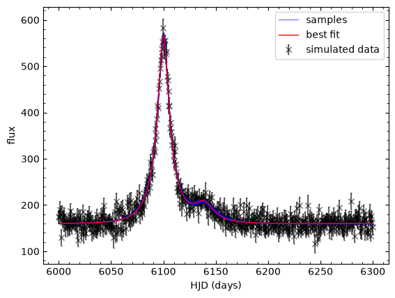
# Plot the lightcurve
plt.close(8)
plt.figure(8)

######################
# EXERCISE: BinarySourceE8.txt PART: 3
#---------------------
# Your code goes here

# Plot the data
plt.errorbar(time, flux, yerr=flux_err,
             fmt='x',
             ecolor='k',
             capsize=1,
             color='k',
             alpha=0.6,
             zorder=0,
             label='simulated data'
             )

chi2_state = np.zeros(nwalkers)
FS1_state = np.zeros(nwalkers)
FS2_state = np.zeros(nwalkers)
FB_state = np.zeros(nwalkers)
for i in range(nwalkers):
    chi2_state[i], FS1_state[i], FS2_state[i], FB_state[i] = binary_source_chi2(final_state[i],
                                                                                model1,
                                                                                model2,
                                                                                data,
                                                                                return_fluxes=True
                                                                                )

# find the minimum chi2 sample
best = np.argmin(chi2_state)
theta_best = final_state[best]
print('best fit parameters:', theta_best)

def plot_sample(theta, model1, model2, chi2, FS1, FS2, FB, color='k', alpha=0.1, label='_', zorder=0, ms=1):
    """Plot the model lightcurve"""
    model1.parameters.t_0 = theta[0]
    model1.parameters.u_0 = theta[1]
    model1.parameters.t_E = theta[2]
    model2.parameters.t_0 = theta[3]
    model2.parameters.u_0 = theta[4]
    model2.parameters.t_E = theta[5]

    F_model = model1.get_magnification(T) * FS1 + model2.get_magnification(T) * FS2 + FB

    plt.plot(T, F_model, color=color, linestyle='-', lw=1, alpha=alpha, label=label, zorder=zorder, ms=ms)

# Plot the model
for i in np.linspace(0, nwalkers-1, 10, dtype=int):
    if i==0:
        label = 'samples'
    else:
        label = '_samples'

    plot_sample(final_state[i],
                model1,
                model2,
                chi2_state[i],
                FS1_state[i],
                FS2_state[i],
                FB_state[i],
                color='b',
                alpha=0.5,
                zorder=1,
                label=label,
                ms=3
                )

plot_sample(theta_best,
            model1,
            model2,
            chi2_state[best],
            FS1_state[best],
            FS2_state[best],
            FB_state[best],
            color='r',
            label='best fit',
            zorder=2,
            alpha=1
            )


plt.legend()
plt.ylabel('flux')
plt.xlabel('HJD (days)')
######################

plt.show()
best fit parameters: [6.09997812e+03 2.50392908e-01 2.10586185e+01 6.13868403e+03
 4.48374060e-01 2.15985580e+01]
Any parameters that show diagonal samples in the 2D posteriors of the corner plot.
Binary source events can throw a real spanner in the works when it comes to event modelling. Binary sources complicate what is already a very complicated analysis process and the binary source model is full of correlated parameters that make it hard to determine the true values precisely. Not only can they mimic caustic purturbations with a finite source effect, but they can also mess with colour-colour inference between observatories such as contemporaneous space-based observations, or late-time follow-up lens-flux and astrometric observations. With binaries possibly making up 40% or more of the stars in the Galactic centre (Gautam et al., 2024; McTier, Kipping, & Johnston, 2020), this potential complication is not one that should be ignored.
Having a binary source in a microlensing event can double the number of parameters in our models, which has a dramatic impact on compute time. If we are calling a magnification function for each source, then the compute time roughly doubles for each model evaluation, as the magnification function is usually the most computationally intensive piece of microlensing event-modelling code. Besides which, higher dimensions of parameter space simply take longer to explore.
These real costs are part of the reason for why microlensing simulations, to date, mostly ignore binary sources. Recent work by the PopSyCLE team (Abrams et al., 2025) found that, using their population models, 55% of observed microlensing events involve a binary system;
14.5% wth a single source and muptiple lenses,
31.7% with multiple sources and a single lens, and
8.8% with multiple sources and multiple lenses.
This paper is well worth a read, if you have the time.
Exercise 10
Which binary-lens models do you think would have degenerate, binary-source, counter parts?
Binary-lens models that do not have sharp perturbations from the packzynski curve; i.e., those with a large finite-source effect or without caustic crossings
Recent simulations by Sangtarash & Yee (2025) demonstrated that, for Roman-like cadences, the binary-source/wide-orbit-planet degeneracy is most persistent when \(\rho\) is large (which typically occurs in events with small \(\theta_{\rm E}\)) or \(q\) is small, as the likelihoods of the models do not differ significantly in these cases; we can infer that, in general, lower-mass objects make this degeneracy harder to resolve.
As a closing statement for this notebook lets simplify what we have learned to this TLDR:

Next steps#
Well, you've been warned. Now let's move on to something else. Maybe to one of these:
Binary lenses (comming soon - see dev brach)
Higher-order effects (release TDB)
The Galactic model (release TDB)
Okay, bye. I'll see you there.